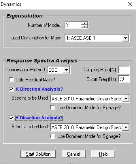
A Response Spectra Analysis may be performed after the dynamic analysis to obtain forces, stresses and deflections. In general, the response spectra analysis procedure is based on the assumption that the dynamic response of a structural model can be approximated as a summation of the responses of the independent dynamic modes of the model.
To Perform a Response Spectra Analysis
Note
To Include Response Spectra Analysis Results in a Load Combination
Note
The response spectra represent the maximum response of any single degree of freedom (SDOF) system to a dynamic base excitation. The usual application of this method is in seismic (earthquake) analysis. Earthquake time history data is converted into a "response spectrum". With this response spectrum, it is possible to predict the maximum response for any SDOF system. By "any SDOF system", it is meant a SDOF system with any natural frequency. "Maximum response" means the maximum deflections, and thus, the maximum stresses for the system.
In the response spectra analysis procedure, each of the model's modes is considered to be an independent SDOF system. The maximum responses for each mode are calculated independently. These modal responses are then combined to obtain the model's overall response to the applied spectra.
The response spectra method enjoys wide acceptance as an accurate method for predicting the response of any structural model to any arbitrary base excitation, particularly earthquakes. Building codes require a dynamics based procedure for some structures. The response spectra method satisfies this dynamics requirement. The response spectra method is easier, faster and more accurate than the static procedure so there really isn't any reason to use the static procedure.
If you wish to learn more about this method, an excellent reference is Structural Dynamics, Theory and Computation by Dr. Mario Paz (1991, Van Nostrand Reinhold).
If a response spectra analysis is solved using modal frequency values that fall outside the range of the selected spectra, RISA will extrapolate to obtain spectral values for the out-of-bounds frequency. If the modal frequency is below the smallest defined spectral frequency, a spectral velocity will be used for the modal frequency that will result in a constant Spectra Displacement from the smallest defined spectral frequency value. A constant spectral displacement is used because modes in the “low” frequency range will tend to converge to the maximum ground displacement. If the modal frequency is above the largest defined spectral frequency, a spectral velocity will be used for the modal frequency that will result in a constant Spectra Acceleration from the largest defined spectral frequency value. A constant spectral acceleration is used because modes in the “high” frequency range tend to converge to the maximum ground acceleration (zero period acceleration).
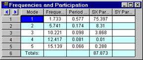
The mass participation factors reported on the Frequencies Spreadsheet reflect how much each mode participated in the Response Spectra Analysis solution. Remember that the RSA involves calculating separately the response for each mode to the applied base excitation represented by the spectra. Here is where you can tell which modes are important in which directions. Higher participation factors indicate more important modes. The participation factor itself is the percent of the model's total dynamic mass that is deflecting in the shape described by the particular mode. Thus, the sum of all the participation factors in a given direction can not exceed 100%.
The amount of participation for the mode may also reflect how much the mode moves in the direction of the spectra application. For example, if the 1st mode represents movement in the global Y direction it won't participate much, if at all, if the spectra is applied in the global X direction. You can isolate which modes are important in which directions by examining the mass participation.
Note
There are three choices for combining your modal results: CQC, SRSS, or Gupta. In general you will want to use either CQC or Gupta. For models where you don’t expect much rigid response, you should use CQC. For models where the rigid response could be important, you should use Gupta. An example of one type of model where rigid response would be important is the analysis of shear wall structures. The SRSS method is offered in case you need to compare results with the results from some older program that does not offer CQC or Gupta.
CQC stands for "Complete Quadratic Combination". A complete discussion of this method will not be offered here, but if you are interested, a good reference on this method is Recommended Lateral Force Requirements and Commentary, 1999, published by SEAOC (Structural Engineers Assoc. of Calif.). In general, the CQC is a superior combination method because it accounts for modal coupling quite well.
The Gupta method is similar to the CQC method in that it also accounts for closely spaced modes. In addition, this method also accounts for modal response that has “rigid content”. For structures with rigid elements, the modal responses can have both rigid and periodic content. The rigid content from all modes is summed algebraically and then combined via an SRSS combination with the periodic part which is combined with the CQC method. The Gupta method is fully documented in the reference, Response Spectrum Method, by Ajaya Kumar Gupta (Published by CRC Press, Inc., 1992).
The Gupta method defines lower ( f 1 ) and upper ( f 2 ) frequency bounds for modes containing both periodic and rigid content. Modes that are below the lower bound are assumed to be 100% periodic. Modes that are above the upper bound are assumed to be 100% rigid.
A response spectra analysis involves calculating forces and displacements for each mode individually and then combining these results. The problem is both combination methods offered (SRSS and CQC) use a summation of squares approach that loses the sign. This means that all the results are positive, except reactions, which are all negative as a result of the positive displacements.
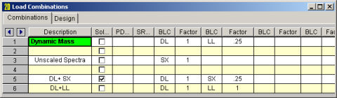
Because the RSA results are unsigned you cannot directly add the results to other static loads in you model. One way around this is to treat the RSA results as both positive and negative by manually providing the sign. Using two combinations for each RSA result, one with a positive factor and the other with a negative factor you can capture the maximum deflections, stresses and forces when combining with other loads. See Load Combinations with RSA Results for an example.
The mass participation may indicate that a model is dominated by a single mode in a direction. You may base the signs for the final combined RSA results on the signs for the RSA for this single dominant mode by checking the box that says “Use Dominant Mode for Signage?”. When that option is selected then the Mode that that the highest mass participation in that direction will be considered to be the dominant mode.
Because of the statistical method used to combine the results , response spectra results can be confusing or misleading to engineers that are not familiar with the process. The confusion is usually associated with the fact any single response spectra result is correct, but that it is not known whether the sign of that result should be positive or negative. This results in a number of limitations that should be considered when using response spectra analysis.
Statics: By default with an RSA solution the results will not obey statics, due to the nature of combining the modes via SRSS, CQC, etc. Thus, if you view the reactions, member forces, etc., the model will not obey statics. If the model has a "dominant" mode in the given direction then the normal path forward would be to select the Use Dominant Mode for Signage? checkbox when solving for the dynamic solution.
For additional advice on this topic, please see the RISA Tips & Tricks webpage at risa.com/post/support. Type in Search keywords: Response Spectra Reactions Satisfy Statics.
Deflected Shape: By default with an RSA solution the results will not obey statics, due to the nature of combining the modes via SRSS, CQC, etc. Thus, if you view the deflected shape you will see that the deflected shape looks odd. Similar to the "Statics" limitation above, one possible path forward is to use the Use Dominant Mode for Signage? checkbox when solving your dynamic solution.
For additional advice on this topic, please see the RISA Tips & Tricks webpage at risa.com/post/support. Type in Search keywords: Response Spectra Reactions Satisfy Statics.
Plate and Wall Contours: Plate contours are not presented to the user for RSA load combination unless the Use Dominant Mode for Signage? option has been chosen. This is because the results can be misleading due to the "Statics" issue described above.
Wall Panel Reactions: Wall Panel reactions consist of a number of internal nodal reactions that are then summed together across the wall. Since the signs of those reactions are unknown, the reactions for each Wall Panel cannot be correctly calculated. There are two methods of dealing with this issue:
Note:
Internal Force Summation Tools : Because the Internal force summation tool relies on plate corner forces, these results are not available for wall panels for any load combination which contains RSA results. Internal force summation tools may be used on other portions of the model. However, they will face the same issue that is described under the "Statics" limitation above. For that reason the results are suppressed unless the Use Dominant Mode for Signage? option has been chosen.
This is the frequency used by the Gupta method to calculate the upper bound for modes having periodic and rigid content. The “rigid frequency” is defined as “The minimum frequency at which the spectral acceleration becomes approximately equal to the zero period acceleration (ZPA), and remains equal to the ZPA”. If nothing is entered in this field, the last (highest) frequency in the selected response spectra will be used.
For seismic response, the typical cutoff frequency would be 33 Hz.
The damping ratio entered here is used in conjunction with the CQC and Gupta combination methods. This single entry is used for all the modes included in the RSA, an accepted practice. A value of 5% is generally a good number to use. Typical damping values are:
2% to 5% for welded steel
3% to 5% for concrete
5% to 7% for bolted steel, wood
The most difficult part of the entire RSA procedure is normally calculating the scaling factor to be used when including the RSA results in a load combination.
The ASCE 7 uses a particular “shape” for it’s spectra (See Figure 11.4-1), but the parameters SDS and SD1 make it specific to a particular site. However, the ASCE 7 imposes several requirements regarding the minimum design values. ASCE 7-16 Section 12.9.1.4.1 specifies a modification factor, V/Vt( ASCE 7-10 Section 12.9.4.1 specifies a modification factor, 0.85*V/Vt), that may be used to scale the response spectra results to something less than or equal the base shear calculated using the static procedure (ASCE 7 Sect. 12.8).
The static base shear (V) is calculated using the equations in ASCE 7-16 Sect. 12.8.1
Note that there are limiting values for the static base shear in ASCE 7-16 equations 12.8-3 through 12.8-6.
Therefore, in order to calculate the proper scaling factor, we need to know what the unscaled RSA base shear (this is called the Elastic Response Base Shear in the IBC) is, and we also need to calculate the value of "V" (static base shear). The calculation of V isn't particularly difficult because the two values that present the biggest problem in this calculation (T and W) are provided by RISA. To calculate the value of W, simply solve a load combination comprised of the model seismic dead weight. This almost certainly will be the same load combination you used in the Dynamics settings for the Load Combination for Mass. The vertical reaction total is your "W" value.
The T value is simply the period associated with the dominant mode for the direction of interest. For example, if you're calculating the scaling factor for a Z-direction spectra, determine which mode gives you the highest participation for the Z direction RSA. The period associated with that mode is your T value. Note that there are limiting values for T, see ASCE 7-16 section 12.8.2.
Calculating the unscaled RSA base shear also is very straightforward. Just solve a load combination comprised of only that RSA, with a factor of 1.
Example:
Scale Factor = (V / Unscaled RSA base shear)
You would do this calculation to obtain the scaling factors for all the directions of interest (X, Y and/or Z). Unless the model is symmetric the fundamental period for each direction is probably different. Be sure to use the proper value for "T" for the direction being considered.
Note: The ASCE 7 has additional requirements for vertical seismic components. (See ASCE 7-16 section 12.4.2.2).
You may have the 1997 UBC spectra generated automatically by selecting "UBC 97, Parametric Design Spectra" for your RSA. The Ca and Cv seismic coefficients are needed to calculate the values for the UBC ’97 spectra. See Figure 16-3 in the UBC for the equations used to build the spectra. See Tables 16-Q and 16-R to obtain the Ca and Cv values. The default values listed are for Seismic Zone 3, Soil Type “Se” (Soft Soil Profile). These values can be edited in the Seismic tab of Model Settings.
You may have the 2000 IBC spectra generated automatically by selecting "IBC 2000, Parametric Design Spectra" for your RSA. The SDS and SD1 seismic coefficients are needed to calculate the values for the IBC 2000 spectra. See Figure 1615.1.4 in the IBC for the equations used to build the spectra. See section 1615.1.3 to obtain the SDS and SD1 values.These values can be edited in the Seismic tab of Model Settings.
You may have the 2005 ASCE spectra generated automatically by selecting "ASCE 2005, Parametric Design Spectra" for your RSA. The SDS, SD1, and TL seismic coefficients are needed to calculate the values for the ASCE 2005 spectra. See Figure 11.4-1 in ASCE-7 2005 for the equations used to build the spectra. See section 11.4.4 to obtain the SDS and SD1 values and Figures 22-15 thru 22-20 for the TL value. These values can be edited in the Seismic tab of Model Settings.
You may have the 2010 ASCE spectra generated automatically by selecting "ASCE 2010, Parametric Design Spectra" for your RSA. The SDS, SD1, and TL seismic coefficients are needed to calculate the values for the ASCE 2010 spectra. See Figure 11.4-1 in ASCE-7 2010 for the equations used to build the spectra. See section 11.4.4 to obtain the SDS and SD1 values and Figures 22-12 thru 22-16 for the TL value. These values can be edited in the Seismic tab of Model Settings.
You may have the 2016 ASCE spectra generated automatically by selecting "ASCE 2016, Parametric Design Spectra" for your RSA. The SDS, SD1, and TL seismic coefficients are needed to calculate the values for the ASCE 2016 spectra. See Figure 11.4-1 in ASCE-7 2016 for the equations used to build the spectra. See section 11.4.5 to obtain the SDS and SD1 values and Figures 22-14 thru 22-17 for the TL value. These values can be edited in the Seismic tab of Model Settings.
You may have the 2005 NBC spectra generated automatically by selecting "NBC 2005 Parametric Design Spectra" for your RSA. The Site Class and the Savalues are needed to calculate the values for the NBC 2005 spectra. Please see section 4.1.8.4(7) to obtain the Sa values and Table 4.1.8.4(A) for the Site Class. Please see section 4.1.8.4(7) for the equations used to build the spectra.These values can be edited in the Seismic tab of Model Settings.
You may have the 2010 NBC spectra generated automatically by selecting "NBC 2010 Parametric Design Spectra" for your RSA. The Site Class and the Savalues are needed to calculate the values for the NBC 2010 spectra. Please see section 4.1.8.4(7) to obtain the Sa values and Table 4.1.8.4(.A) for the Site Class. Please see section 4.1.8.4.(7) for the equations used to build the spectra.These values can be edited in the Seismic tab of Model Settings.
You may have the 2015 NBC spectra generated automatically by selecting "NBC 2015 Parametric Design Spectra" for your RSA. The Site Class and the Savalues are needed to calculate the values for the NBC 2015 spectra. Please see section 4.1.8.4(7) to obtain the Sa values and Table 4.1.8.4(.A) for the Site Class. Please see section 4.1.8.4.(7) for the equations used to build the spectra.These values can be edited in the Seismic tab of Model Settings.
You may add your own spectra to the database and edit and delete them once they are created. You can add/edit spectra data pairs in any configuration by choosing between Frequency or Period and between the three spectral values. You may also choose to convert the configuration during editing. At least two data points must be defined. Log interpolation is used to calculate spectra values that fall between entered points. Make sure that all of the modal frequencies in your model are included within your spectra.
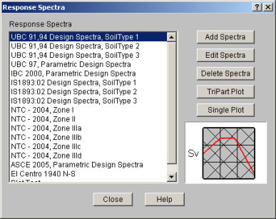
To Add or Edit a Spectra
Note
This plot is a convenient logarithmic representation of all the values of interest in the response spectra definition.
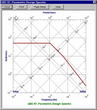
These values are as follows:
Frequency (f)
Period (T)
Pseudo Velocity (Sv)
Pseudo Acceleration (Sa)
Pseudo Displacement (Sd)
The relationships between these values (for the undamped case) is as follows:
T = 1. / f
Sv = Sd * 2πf = Sa / 2πf
For the tripartite plot, the frequency values are plotted along the bottom with the reciprocal period values displayed along the top. The ordinate axis plots the Sv values (labeled on the left side) and the diagonal axes plot the Sa (lower left to upper right) and Sd (upper left to lower right) values.
The spectra data itself is represented with the thick red line. Therefore, to determine the Sv, Sa or Sd value for a particular frequency or period, locate the desired period or frequency value along the abscissa axis and locate the corresponding point on the spectra line. Use this point to read off the Sv, Sa and Sd values from their respective axes. Remember, all the axes are logarithmic!
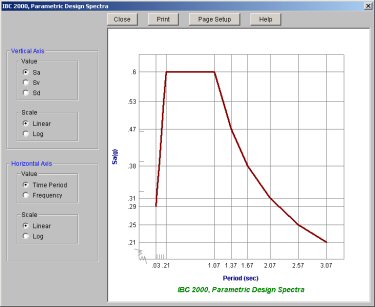
This plot is a Response spectra representation that is given in the building codes. The vertical axis can plot the spectra using Pseudo-Acceleration, Pseudo-Velocity, or Pseudo Displacement on a vertical or logarithmic scale. The horizontal axis will plot the Period or Frequency using a Linear or Logarithmic scale.
These values are as follows:
Frequency (f)
Period (T)
Pseudo Velocity (Sv)
Pseudo Acceleration (Sa)
Pseudo Displacement (Sd)
The relationships between these values (for the undamped case) is as follows:
T = 1. / f
Sv = Sd * 2πf = Sa / 2πf
The spectra data itself is represented with the thick red line. Therefore, to determine the Sv, Sa or Sd value for a particular frequency or period, locate the desired period or frequency value along the horizontal axis and locate the corresponding point on the spectra line. Use this point to read off the Sv, Sa and Sd values from their vertical axis.